Performing a parallel pump-probe RT-TDSCF simulation in ReSpect is a simple three-step process. The first two steps include

respect --scf   --inp=my-input-file --nt=4 --scratch=/path/to/scratch/directory
respect --tdscf --inp=my-input-file --nt=4 --scratch=/path/to/scratch/directory

The first call of respect with the argument --scf starts a time-independent SCF calculation, which is a necessary prerequisite for the following RT-TDSCF calculation. The second call of respect with the argument --tdscf actually performs the pump-probe RT-TDSCF simulation.

The other arguments mandatory to respect are

• --inp
  specifies a name of the input file;

• --nt
  specifies the number of physical cores required for parallel execution;

• --scratch
  specifies a path to the scratch directory.

The input file my-input-file.inp should contain the input block scf: with some SCF-specific keywords, and the input block tdscf: with some TDSCF-specific keywords. A comprehensive list of all keywords can be found for SCF here and for TDSCF here. A simple example of my-input-file.inp looks like

#non-relativistic 1c Hartree-Fock calculation of H2O molecule
scf:

    geometry:
        O    0.000000    0.000000    0.000000
        H    0.000000    0.000000    0.940000
        H    0.903870    0.000000   -0.258105

    method: hf
    basis:  ucc-pvdz

    charge:        0
    multiplicity:  1
    nc-model:      point
    maxiterations: 30
    convergence:   1.0e-7


#RT-TDSCF calculation with two external fields: an enveloped cos^2 pump of 
#amplitude 0.02[a.u.] along y-direction, and a delta-type probe of amplitude 
#0.001[a.u.] along x-direction. The pump field has additional attributes such 
#as carrier frequency and carrier width with maximum at time 129[a.u.].
tdscf:
   spectroscopy:     eas
   time-steps:       2516 x 0.5

   field:
         model:      cos2
         amplitude:  0.02
         direction:  0.0 1.0 0.0
         frequency:  0.3662   #carrier frequency = first excitation energy
         width:      258.0    #carrier width = 15 cycle pulse (15*2*pi/freq)
         inittime:   129.0    #carrier maximum = carrier width/2

   field2:
         model:      delta
         amplitude:  0.001
         direction:  1.0 0.0 0.0
         inittime:   258.0

There are several important aspects associated with the pump-probe RT-TDSCF simulations

• the inittime: of the probe pulse (field2:) should be equal or larger than the width: (i.e. duration) of the pump pulse (field:). This is related to a non-overlapping regime assumed in our simulations. In addition, ensure that inittime: is half the width: for model:cos2 field, and they are integer multiples of the time-step used, which is 0.5 for the above example.

• ensure that the pump field width: is chosen roughly to be equal to an integer number of cycle. Given the example above, 15 cycles of frequency:0.3662 has a width: of \(15*2\pi/0.3662 = 257.2 \approx 258\).

• it is necessary to perform three independent pump-probe RT-TDSCF simulations with the probe field (field2:) oriented along three perpendicular Cartesian directions.
  The easiest way to accomplish this requirement is to set the keyword direction: in the input block field2: to an unit vector along the x-axis as

direction:  1.0  0.0  0.0

or to an unit vector along the y-axis as

direction:  0.0  1.0  0.0

or to an unit vector along the z-axis as

direction:  0.0  0.0  1.0

and rerun the pump-probe RT-TDSCF simulation for each direction. Importantly, save the pump-probe TDSCF output files with specific suffixes -- _pp_x.out_tdscf for x-direction, _pp_y.out_tdscf for y-direction, and _pp_z.out_tdscf for z-direction. These name-specific files will be required for a final post-processing of the time-domain signal and visualisation of pump-probe absorption spectra (see text below).

• to maintain the same spectral resolution for pump-probe RT-TDSCF as for ordinary probe-only RT-TDSCF, add the step count for the onset of the probe pulse to the total number of steps. For example, if probe-only RT-TDSCF was done with time-steps:2000 x 0.5, the corresponding pump-probe RT-TDSCF with the probe applied at inititime:258 should have time-steps:2516 x 0.5, where 2516 = (2000 + 258/0.5).

Having the three pump-probe TDSCF outputs files, named for instance as  my-output_pp_x.out_tdscf, my-output_pp_y.out_tdscf and my-output_pp_z.out_tdscf, we are ready to perform the last simulation step aimed at isolating the effect of probe pulse only. This requires to remove the entire block field2: from the section tdscf: in the input file my-input-file.inp

tdscf:
   spectroscopy:     eas
   time-steps:       2516 x 0.5

   field:
         model:      cos2
         amplitude:  0.02
         direction:  0.0 1.0 0.0
         frequency:  0.3662   #carrier frequency = first excitation energy
         width:      258.0    #carrier width = 15 cycle pulse (15*2*pi/freq)
         inittime:   129.0    #carrier maximum = carrier width/2

and rerun one pump-only RT-TDSCF simulation with the command

respect --tdscf --inp=my-input-file --nt=4 --scratch=/path/to/scratch/directory

Importantly, save the pump-only TDSCF output file with the specific suffix -- my-output_p.out_tdscf. Finally, the pump-probe electronic absorption spectrum can be generated and visualized with the help of spectrum.py

/path/to/ReSpect/util/spectrum.py --files=my-output --spectroscopy=tas --plot

In addition to the spectral plot, the script will also generate two files;  my-output.out_spectrum_tas containing all datapoints of the frequency domain, and my-output.out_peaks_tas containing datapoints above the threshold 10^-7 and information about the post-processing settings, relevant physical constants, and spectral resolution. All arguments to the script spectrum.py can be listed by the command

/path/to/ReSpect/util/spectrum.py --help

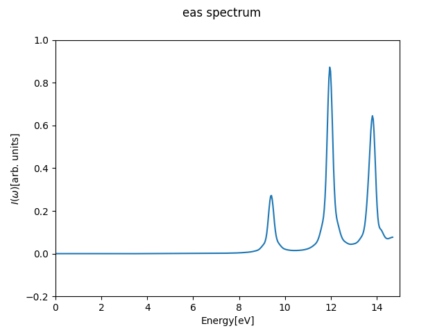
The final pump-probe transient absorption spectrum (TAS) of water should look like

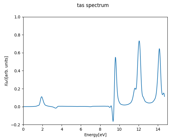
Note that the spectrum has several distinct features from the ordinary electronic absorption spectra (EAS)

There are several important and worth-to-remember aspects associated with the syntax of ReSpect input files, namely

• the input is case-insensitive
  This means that the program does not distinguish between uppercase and lowercase letters.

• the input is insensitive to the number of blank lines and/or comment lines
  All comments begin with the number sign (#), can start anywhere on a line and continue until the end of the line.

• the input is compliant with the dictionary syntax of the YAML markup language
  This means that each input line is represented either by a single block: statement or by a simple keyword:value pair, such as

block1:
    keyword1: value1 
    keyword2: value2  
    ...
    block2: 
      keyword3: value3
      keyword4: value4
      ...
    block3: 
           keyword5: value5
           keyword6: value6
           ...

It is essential to remember that all members of one block: are lines beginning at the same indentation level. Whitespace indentation is used to denote the block structure; however, tab characters are never allowed as indentation. The only exception to the YAML-based input syntax is the block geometry: which utilizes a simple xyz format for the molecular geometry specification.

Q: How to scale the speed of light in the RT-TDSCF calculation?

Set the cscale option in the SCF calculation. The scaling value is then automatically transferred to the RT-TDSCF calculation.

Q: Is it possible to scale spin-orbit interaction in the RT-TDSCF calculation?

No. Currently this feature is not supported.

Q: Is there a way to launch RT-TDSCF calculations without the need to explicitly setup the scratch path by "--scratch=/path/to/scratch/directory"?

Yes, the argument "--scratch=/path/to/scratch/directory" can be saved to the file .respectrc in your home directory. If both the file and the command line argument exist, then ReSpect takes the scratch directory setting from the command line.

Q: How to restart a RT-TDSCF calculation?

RT-TDSCF calculations can be restarted simply by creating the symbolic link to the data file of the previous job

ln -sf my-old-job.50 my-new-job.50

and by adding an extra argument --restart to the command line when restarting new job

/path/to/ReSpect/respect --tdscf --inp=my-new-job --restart

The restart process collects and prints to the output file my-new-job.out_tdscf all relevant RT-TDSCF data generated in the previous run.

Q: Is it possible to recover a RT-TDSCF job from a scratch directory?

If the ReSpect job for any reason fails and the scratch directory is still accessible, it is possible to recover the failed calculation. After running the command

/path/to/ReSpect/respect --recover-job=/path/to/scratch/directory

file respect_checkpoint_file.50 will be created in the current directory. Using this file, you can now restart the RT-TDSCF calculation as described in the tip How to restart a RT-TDSCF calculation?.