Performing a parallel relativistic calculation of band strucutres of 1D, 2D, and 3D periodic systems is done in two steps, i.e. by executing two distinct commands to run the respect code from a directory containing my-input-file.inp. The first command

respect --pscf --inp=my-input-file --nt=4 --scratch=/path/to/scratch/directory

of respect with the argument --pscf performs the periodic self-consistent field (pSCF) optimization of the ground-state crystalline orbitals (and the density matrix) in an iterative manner. Converged orbitals can then be used for property calculations, e.g. the electric-field gradient (EFG) tensor, or for obtaining the band-structure ("spaghetti") diagrams. These diagrams are obtained from the second run of respect by executing

respect --pscf-bands --inp=my-input-file --nt=4 --scratch=/path/to/scratch/directory

The other arguments mandatory to respect are

• --inp
  specifies a name of the input file;

• --nt
  specifies the number of physical cores required for OpenMP parallel execution;

• --scratch
  specifies a path to the scratch directory.

The input file my-input-file.inp should contain the input block pscf: to control the parameters of the pSCF section for the ground-state optimization and the input block pscf-bands: to control the parameters of the subsequent bands run. A comprehensive list of all pSCF keywords can be found here and for pscf-bands here. A simple example of my-input-file.inp is

#periodic DFT calculation of 2D graphene, employing the non-relativistic
#1c Kohn-Sham Hamiltonian with PBE functional using the RI-J approximation
#for the 2-electron Coulomb interactions
pscf:
     geometry:
          C     0.000000   0.000000   0.000000
          C     1.231859   0.711214   0.000000
     lattice:
          a1:   1.231859  -2.133643
          a2:   1.231859   2.133643

     kmesh:          33x33x1
     basis:          ucc-pvdz
     method:         ks/pbe
     initmo:         atomic
     nc-model:       point
     maxiterations:  30
     convergence:    5.0e-5

     peri:
          threshold:     1.0e-9
          acceleration:  ri-j

     #we use a very small grid here just to make the calculation run faster
     #in most productive calculations, this specification can be omitted
     grid:
          C:   30  86


#the second section sets up the path in k space as well as the mesh for DOS calculation
pscf-bands:
     #these two ways of setting up k points are equivalent
     #kpoints:      2d-hexagonal  50
     kpoints:
       steps:  50
       point:  G  0.00000000  0.00000000  0.00000000
       point:  M  0.50000000  0.00000000  0.00000000
       point:  K  0.33333333  0.33333333  0.00000000
       path:   G-M-K-G
     kmesh:        33x33x1
     print-bands:  2-13
     full-print:   on

After the completion of the pscf-bands calculation, it is possible to visualize the band structures by using the post-processing script plot_band_structure.py, i.e. by running

/path/to/ReSpect/util/plot_band_structure.py --file=my-output-file.out_pscf-bands line

The example input above produces the following band structure

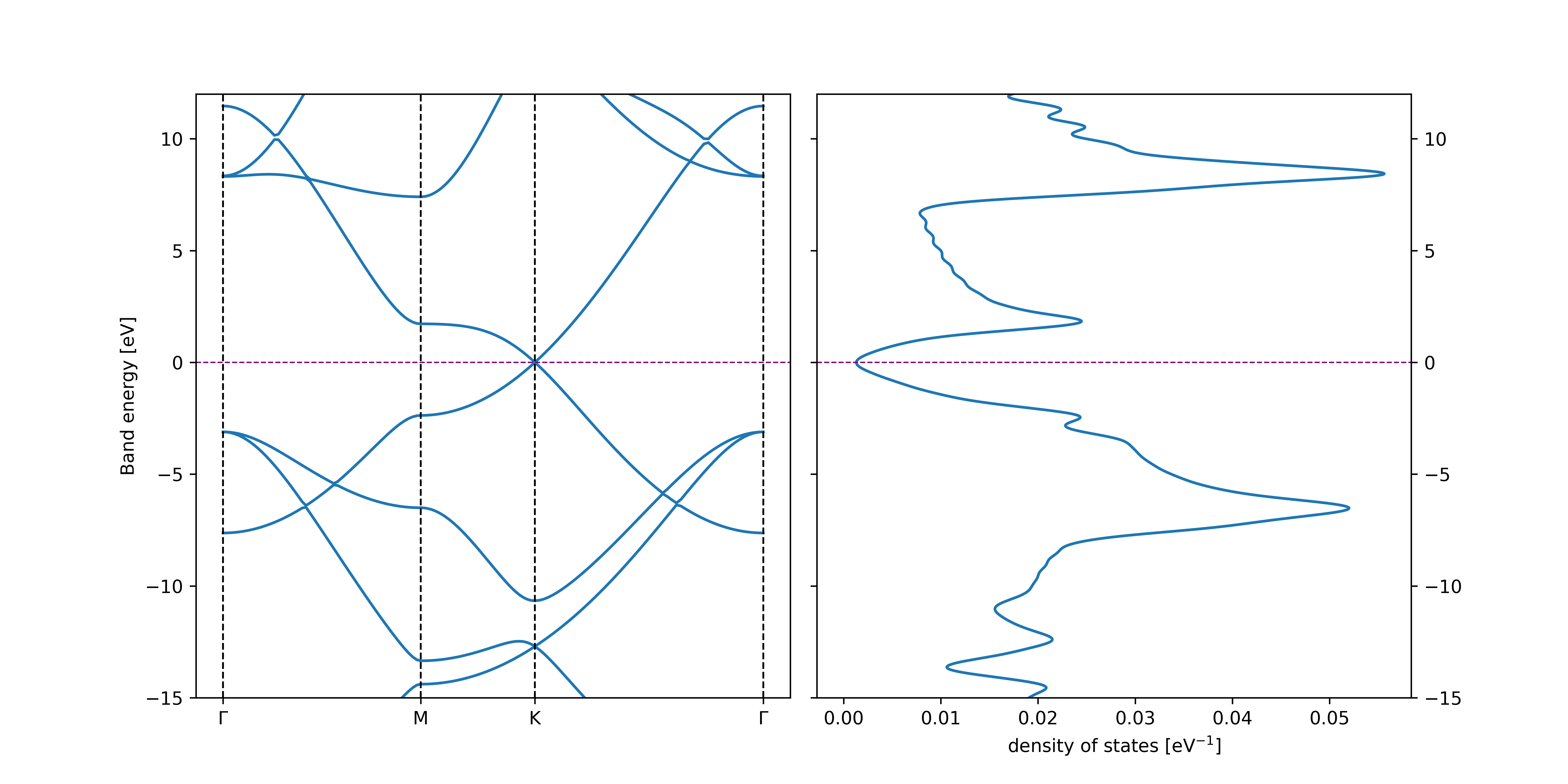
There are a few things to point out when generating band structures and post-processing the pSCF output.

• Calculation of the Density of States (DOS) is automatically activated by specifying the kmesh size in the pscf-bands block. Parameters, such as the energy window or the width of the Gaussians used to replace the Dirac deltas, can optionally be specified by the dos: block. If kmesh is not specified, the DOS calculation is skipped, and only the band structure is produced.

• Note, that only the bands in the range specified by print-bands are printed. Bands outside of this range will not be visible in the plot.

• The plot_band_structure.py script can plot two sets of band structures corresponding to two different calculations using the line2 option as

/path/to/ReSpect/util/plot_band_structure.py -f first.out_pscf-bands line2 -f second.out_pscf-bands

This is useful e.g. when comparing relativistic/nonrelativistic calculations or different basis sets. The script also prints "band delta", i.e. the root-mean-square deviation between the two band structures in the given energy window.

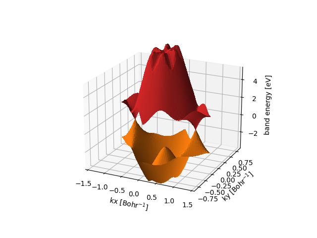
• Keyword full-print triggers the printing of all orbital energies for all k points (in the range given by print-bands). For 2D materials, this can be used to produce 3D surface plots of 2D band structures with the option surface in the command

/path/to/ReSpect/util/plot_band_structure.py -f my-output-file.out_pscf-bands --range="-3.5 5" surface



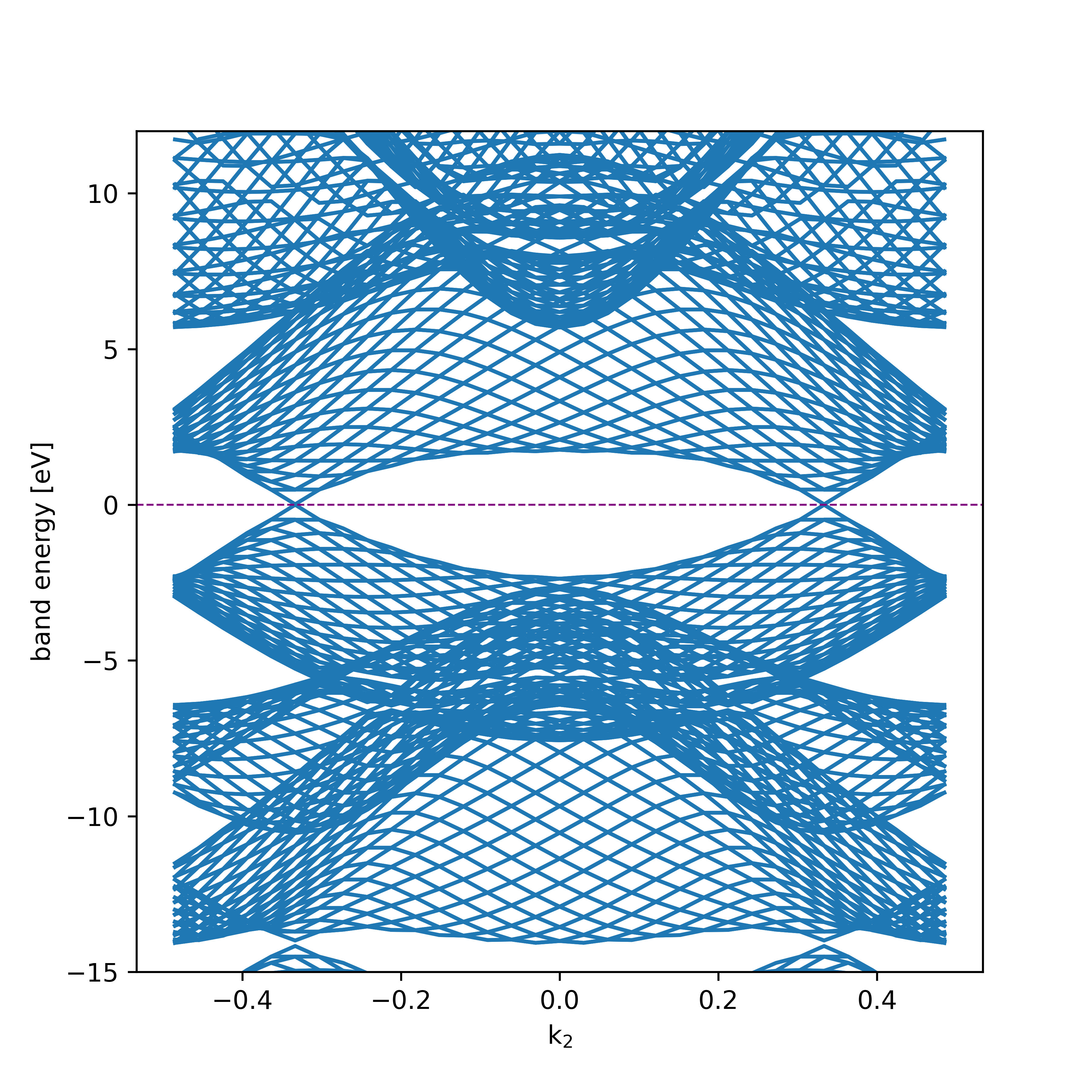
• Likewise, for 2D materials, edge band structure (see page 26 in D. Vanderbilt, Berry phases...) can be constructed using the edge option as

/path/to/ReSpect/util/plot_band_structure.py -f my-output-file.out_pscf-bands --figsize 6 6 edge

For calculating relativistic band structures, it is sufficient to replace a few lines in the input file

method:         mdks/pbe
nc-model:       gauss
cscale:         0.1

The method mdks uses the 4-component Dirac-Kohn-Sham Hamiltonian that includes all relativistic effects (scalar and spin-orbit) variationally. For relativistic calculations, it is recommended to use gauss nucleus model rather than point to avoid having to describe the singularity of the Dirac equation with point-charge potential in finite basis sets.

• Relativistic effects for light atoms (such as carbon) are small, but we can enhance them by downscaling the speed of light with cscale. Likewise, the SOC part of the Hamiltonian can be scaled by using soscale, for instance, it is possible to do purely scalar relativistic calculation by scaling the SOC by a factor of 0 as

soscale:        0.0

• Calculation of the Z₂ invariant is performed automatically for 2D systems when the mdks method is used in the first step (ground-state optimization). The example above produces the following output

Parity of occupied Bloch states at TRIM points
----------------------------------------------
           Band         G           X           Y           R
---------------------------------------------------------------
parity:       1        0.95        0.78       -0.78        0.78
parity:       2        0.95        0.78       -0.78        0.78
parity:       3       -0.95       -0.78        0.78       -0.78
parity:       4       -0.95       -0.78        0.78       -0.78
parity:       5        1.00        1.00       -1.00        1.00
parity:       6        1.00        1.00       -1.00        1.00
parity:       7       -1.00       -1.00        1.00       -1.00
parity:       8       -1.00       -1.00        1.00       -1.00
parity:       9        1.00        1.00       -1.00        1.00
parity:      10        1.00        1.00       -1.00        1.00
parity:      11        1.00       -1.00        1.00       -1.00
parity:      12        1.00       -1.00        1.00       -1.00
---------------------------------------------------------------
product over pairs:    1          -1          -1          -1

Z2 topological invariant =  1

which shows that graphene is a 2D topological insulator exhibiting the quantum spin Hall effect. Note, that this technique will only work for centrosymmetric 2D materials (i.e. with the space inversion symmetry).

• We can use the line2 command in the plot_band_structure.py script to plot both the nonrelativistic and relativistic band structures for comparison

There are several important aspects associated with the input syntax, namely

• the input is case-insensitive
  This means that the program does not distinguish between uppercase and lowercase letters.

• the input is insensitive to the number of blank lines and/or comment lines
  All comments begin with the number sign (#), can start anywhere on a line and continue until the end of the line.

• the input is compliant with the dictionary syntax of the YAML markup language
  This means that each input line is represented either by a single block: statement or by a simple keyword:value pair, such as

block1:
    keyword1: value1 
    keyword2: value2  
    ...
    block2: 
      keyword3: value3
      keyword4: value4
      ...
    block3: 
           keyword5: value5
           keyword6: value6
           ...

It is essential to remember that all members of one block: are lines beginning at the same indentation level. Whitespace indentation is used to denote the block structure; however, tab characters are never allowed as indentation. The only exception to the YAML-based input syntax is the block geometry: which utilizes a simple xyz format for the molecular geometry specification.

Q: Is there a way to launch pSCF calculations without the need to explicitly setup the scratch path by "--scratch=/path/to/scratch/directory"?

Yes, the argument "--scratch=/path/to/scratch/directory" can be saved to the file .respectrc in your home directory. If both the file and the command line argument exist, then ReSpect takes the scratch directory setting from the command line.

Q: How to restart an pSCF calculation?

ReSpect offers a rather flexible framework for restarting pSCF as it allows restarting between various Hamiltonians or computational settings. pSCF calculations can be restarted simply by creating the symbolic link to the data file of the previous job

ln -sf my-old-job.50 my-new-job.50

and by adding an extra argument --restart to the command line when restarting new job

respect --restart --pscf --inp=my-new-job --nt=4 --scratch=/path/to/scratch/directory

However, some caution is needed here as the restart process rewrites all the previous pSCF data, both in the output file (my-new-job.out_pscf) as well as in the checkpoint file (my-new-job.50). If needed, make a backup of these files prior to the restart.

Q: Is it possible to recover an pSCF job from a scratch directory?

If the ReSpect job for any reason fails and the scratch directory is still accessible, it is possible to recover the failed calculation. After running the command

respect --recover-job=/path/to/scratch/directory

file respect_checkpoint_file.50 will be created in the current directory. Using this file, you can now restart the pSCF calculation as described in the tip above.