Performing a parallel relativistic calculation of excitation energies and Xray electronic absorption spectra (XAS) with damped-response TDDFT (DR-TDDFT), known also as complex polarization propagator TDDFT (CPP-TDDFT), is a simple two-step process

respect --scf --inp=my-input-file --nt=4 --scratch=/path/to/scratch/directory
respect --cpp --inp=my-input-file --nt=4 --scratch=/path/to/scratch/directory

The first call of respect with the argument --scf performs the self-consistent field (SCF) optimization of ground-state molecular orbitals, which is a necessary prerequisite for the following property calculation. The second call of respect with the argument --cpp actually performs the DR-TDDFT XAS simulation.

The other arguments mandatory to respect are

• --inp
  specifies a name of the input file;

• --nt
  specifies the number of physical cores required for parallel execution;

• --scratch
  specifies a path to the scratch directory.

The input file my-input-file.inp should contain the input block scf: with some SCF-specific keywords, and the input block cpp: with some XAS-specific keywords. A comprehensive list of all keywords can be found for SCF here and for XAS here. A simple example of my-input-file.inp looks like

#SCF section
#DFT calculation of H2S molecule, employing the relativistic 2c
#amfX2C Hamiltonian, PBE0 functional and uncontracted cc-pvdz basis
scf:

    geometry:
        S        0.000000         0.000000         0.000000
        H        0.000000         0.000000         1.336000
        H        1.335103         0.000000        -0.048956

    method: ks-amfX2C/pbe0

    basis:
          H: ucc-pvdz
          S: ucc-pvdz

    charge:        0
    multiplicity:  1
    maxiterations: 30
    nc-model:      gauss
    convergence:   1.0e-7


#DR-TDDFT section
cpp:
    property:      eas
    maxiterations: 30
    convergence:   1.0e-5
   
    #selection of a window of MOs within which excitations can take place 
    mowindow:
      type:      cvs     #core-valence separation 
      occupied:  5-10    #occupied MOs
      virtual:   19-44   #virtual MOs

    units:       ev
    damping:     0.15
    frequencies: 160.0 105x0.25  #105 frequency points with step 0.25 starting from 160 eV

Final output data from the DR-TDDFT calculation are saved in file my-input-file.out_cpp. Of relevance for XAS are absorption intensities, which are listed for all user-selected frequency points in the last column of a table at the bottom of the output file

Freq           Freq          Real part      Imag part    Polarizability     EAS
[au]           [eV]             [au]           [au]          [au]           [au]
----------------------------------------------------------------------------------
5.87989      160.00000        0.03592        0.07647        0.03592        0.04123
5.88908      160.25000        0.06245        0.05555        0.06245        0.03000
5.89827      160.50000        0.06790        0.05500        0.06790        0.02975
5.90745      160.75000        0.05770        0.06513        0.05770        0.03528
5.91664      161.00000        0.02266        0.09042        0.02266        0.04906
..................................................................................
6.79862      185.00000       -0.23809        0.01955       -0.23809        0.01219
6.80781      185.25000       -0.21173        0.01361       -0.21173        0.00850
6.81700      185.50000       -0.19245        0.01023       -0.19245        0.00639
6.82619      185.75000       -0.17749        0.00808       -0.17749        0.00506
6.83537      186.00000       -0.16541        0.00662       -0.16541        0.00415

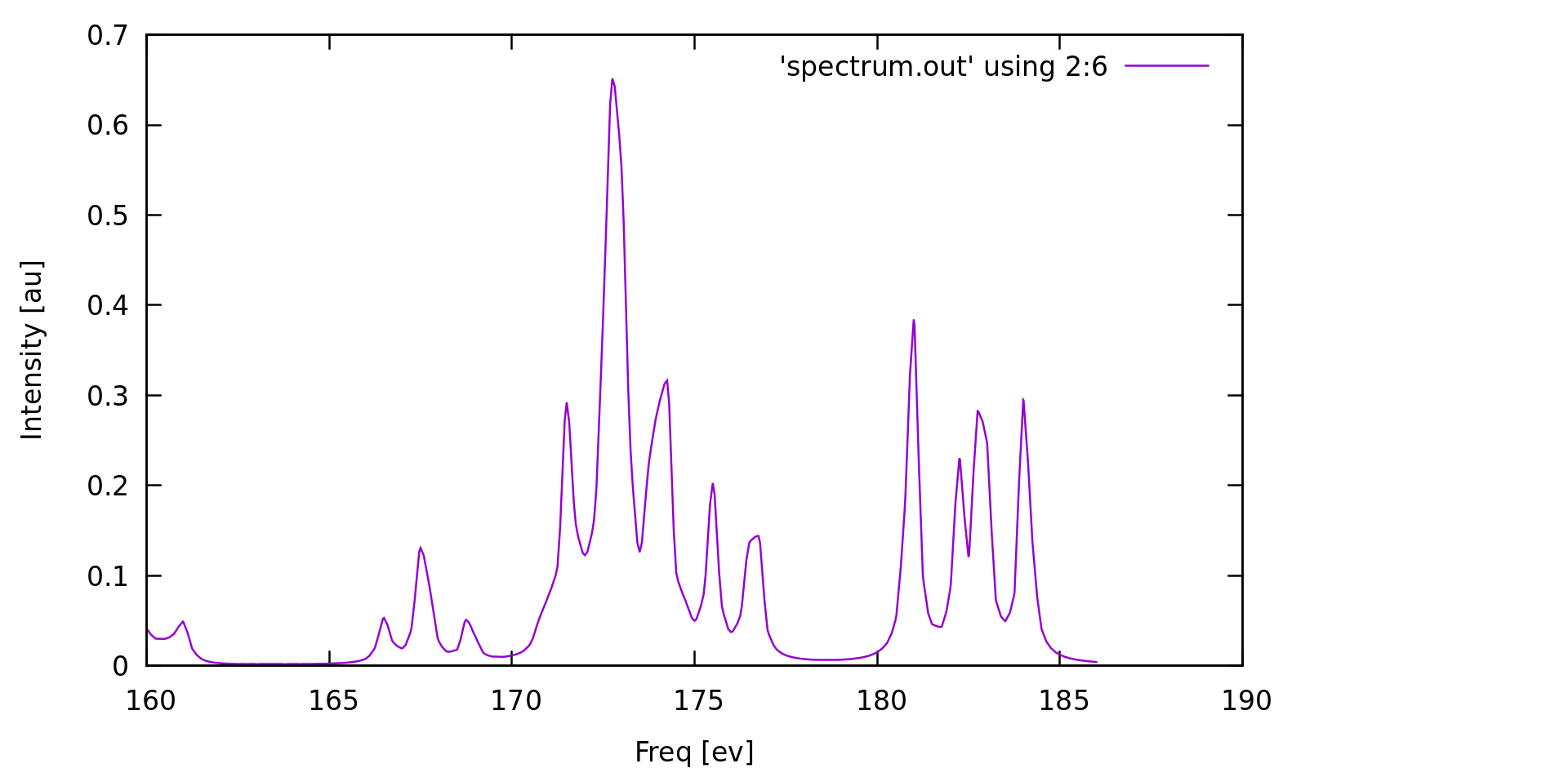
These data can be used to plot the final XAS spectrum. For instance, the simple Linux command grep and the gnuplot program can be used to extract the table and to visualize the XAS spectrum.

grep -A111 'Final isotropic' my-input-file.out_cpp | tail -n +8 > spectrum.out
gnuplot -e "set xlabel 'Freq [ev]'; set ylabel 'Intensity [au]'; plot 'spectrum.out' using 2:6 smooth mcspline w lines; pause -1" 

Finally, note that 105 frequencies from the example above will be treated together. Having more points helps the convergence and enables to cover the whole spectral region of interest. However, adding more points makes the calculation run longer and require more memory, while the convergence is not markedly improved beyond a certain number of points. Therefore, it is recommended to find some compromise and partition the spectral region into several smaller ones containing e.g. 20 to 50 points, and run these few calculations in parallel.

Finally, there are several important aspects associated with the input syntax, namely

• the input is case-insensitive
  This means that the program does not distinguish between uppercase and lowercase letters.

• the input is insensitive to the number of blank lines and/or comment lines
  All comments begin with the number sign (#), can start anywhere on a line and continue until the end of the line.

• the input is compliant with the dictionary syntax of the YAML markup language
  This means that each input line is represented either by a single block: statement or by a simple keyword:value pair, such as

block1:
    keyword1: value1 
    keyword2: value2  
    ...
    block2: 
      keyword3: value3
      keyword4: value4
      ...
    block3: 
           keyword5: value5
           keyword6: value6
           ...

It is essential to remember that all members of one block: are lines beginning at the same indentation level. Whitespace indentation is used to denote the block structure; however, tab characters are never allowed as indentation. The only exception to the YAML-based input syntax is the block geometry: which utilizes a simple xyz format for the molecular geometry specification.

Q: How to scale the speed of light in the DR-TDDFT calculation?

Set the cscale option in the SCF calculation. The scaling value is then automatically transferred to the DR-TDDFT calculation.

Q: Is it possible to scale spin-orbit interaction in the DR-TDDFT calculation?

No. Currently this feature is not supported.

Q: Is there a way to launch DR-TDDFT calculations without the need to explicitly setup the scratch path by "--scratch=/path/to/scratch/directory"?

Yes, the argument "--scratch=/path/to/scratch/directory" can be saved to the file .respectrc in your home directory. If both the file and the command line argument exist, then ReSpect takes the scratch directory setting from the command line.

Q: How to restart a DR-TDDFT calculation?

DR-TDDFT calculations can be restarted simply by creating the symbolic link to the data file of the previous job

ln -sf my-old-job.50 my-new-job.50

and by adding an extra argument --restart to the command line when restarting new job

respect --cpp --inp=my-new-job --nt=4 --scratch=/path/to/scratch/directory --restart

The restart process build on the previously converged or uncoverged solution and starts new iteration cycle. If nothing was stored during a previous calculation (e.g. a job time out occured before it got to the given cartesian component), a calculation will start from the standard initial guess

Q: Is it possible to recover a DR-TDDFT job from a scratch directory?

If the ReSpect job for any reason fails and the scratch directory is still accessible, it is possible to recover the failed calculation. After running the command

respect --recover-job=/path/to/scratch/directory

file respect_checkpoint_file.50 will be created in the current directory. Using this file, you can now restart the DR-TDDFT calculation as described in the tip How to restart a DR-TDDFT calculation?.